Here I will discuss how I created my own car cards and waybills using Microsoft Excel’s spreadsheet software.
Note: this will not be intended to be a detailed tutorial on Excel, or the specific features I’m using; I will show enough to convey how I’m using the feature(s), but for additional details I will refer you to Excel’s documentation or other help sites. It should also be possible to achieve these results using similar tools in other spreadsheet software, but I leave that research to the reader as to how the tools in those softwares may differ from Excel.
Car Cards
The specific design of the car cards and waybills is inspired by the ones we use at the club created and printed using the Ship-It model railroad software. They follow the same dimensions and general form factor, although I have tweaked the design a little to customize it for my own purposes (especially of the shipment waybill insert slips – see below).
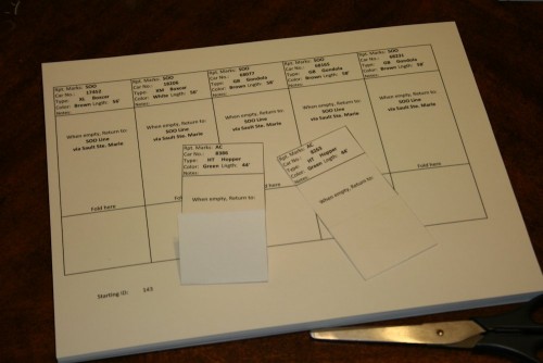
On the car card, the car information goes at the top, with the most important information (identifying reporting mark and number) in the central place of prominence. Other descriptive information such as type, colour and length are included below to assist in visually identifying the car. The Notes field may indicate other special features of the car, or usage restrictions (for example, “Paper service only” on boxcars meant for such).
The bottom of the card is designed to fold up and be taped to form a pocket into which the shipment/routing portion of the paper work (waybill) is inserted.
Below we see the Excel sheet I use for printing out my car cards. It took some tweaking to get the column sizes exactly correct, but otherwise looks pretty straightforward. However, under the hood all of the fields are defined with formulas that pull data from another sheet in the workbook. I didn’t want to copy and past page after page after page of hand-coded car cards (and especially the waybills with their vastly higher number of fields and flopped orientation) so I made one template page, and used Excel lookup functions to pull the data from another sheet, so the car data could be tracked and manipulated far easier in a standard grid format, and any arbitrary range selected for actual printing. In this way, car cards for a large fleet of hundreds of cars can easily be created.
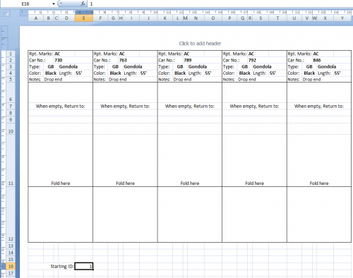
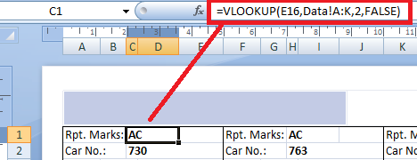
You’ll see in the first image above of the car card template sheet, a “Starting ID” cell below the cards (in cell E16, highlighted). I’m going to use the value in this cell to feed into the Excel lookup functions, which will extract data from the actual roster sheet, and populate it into the fields in the car card template for printing.
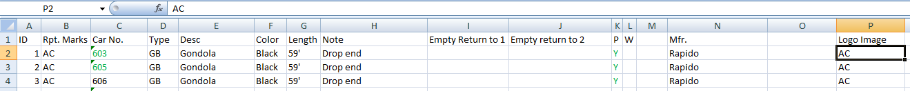
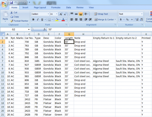
Below is the actual roster information, contained in another sheet within the same workbook. Way easier to read and keep track of, and much more additional notes and information can be added in further columns to the right; our lookup only needs to deal with the first ten columns. Note in particular the first column with the heading “ID”. This is the value we’re going to lookup, and then populate the date from the other columns in the same row into the template sheet for printing.
Excel has several data lookup functions, and the one we want is the “VLOOKUP” function. The VLOOKUP function scans through a specified range of data, looking for a specific value in a particular column. Once that value is found in the search column, it can return a value from another column in that row. The VLOOKUP function in Excel looks like this:
=VLOOKUP( [value],
          [source sheet name]![data columns],
          [column # in data to pull result from],
          [allow approximate matches])
In my case above, we’re pulling the lookup value (the car ID) out of cell E16, so the reference to that cell is the value. (For the subsequent car cards, we want to pull the next several cars in the data sheet, so the lookup value will be the value of (E16)+1, (E16)+2, etc., so if the starting ID is 1, car cards 1 through 5 will be printed.)
The name of my second sheet with the car data is “Data”, and the data is in columns A through K in that sheet. (The VLOOKUP function will scan the first column trying to find the lookup value.)
The last argument should be set to FALSE as we only want an exact match.
Put that all together, and the lookup for the reporting mark field on the first car card looks like this:
One thing to know about the VLOOKUP function in excel, is that if the returned cell in the data sheet is blank, the VLOOKUP function will display that as a 0 in the display cell. For some fields here, like the Notes and Empty return information, I definitely want the cell to be blank if there’s no data, not rendered as zeroes. To protect that, any cell that’s using a VLOOKUP that you want to allow to be blank will need to be wrapped with an Excel IF function, which looks like this:
=IF ([condition], [value if true], [value if false])
In this case, my condition will be if the value from the lookup function is blank (“”), make the cell blank, otherwise insert the returned value. If I do this for the example cell in the image above, it would end up looking like this:
=IF (VLOOKUP(E16,Data!A:K,2,FALSE)="", "", VLOOKUP(E16,Data!A:K,2,FALSE))
… which actually looks far more complicated than it is, since the whole lookup function is pasted in there twice.
Waybills
I also used these tools to create my own custom waybill template. This was a lot more work than the car cards simply owing to the sheer number of fields involved in each waybill compared to the car card, and managing to fit 10 of them per sheet as opposed to 5 per sheet for the car cards. However, it was largely a matter of just taking the time and effort to copy and adjust the lookup functions much as above. While there are quite a number more fields to deal with, and more waybills fit onto a page than the car cards, the general method is exactly the same. Just time consuming to do that many fields. But once it’s done, you have a dynamic template that can easily and quickly create and print out hundreds of different waybills.
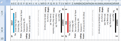
My waybills are “two-cycle” with each one printed on one side of the paper and having two separate moves (generally an empty move and a loaded move), one of which is visible at a time and rotated (between sessions) in the car card pocket to display the second move when the first move is completed. This required printing the second move upside-down to the first – although Excel doesn’t allow you to set the text orientation in a cell to “upside down”. It does however let you do “up” and “down”, so I just designed the waybills sideways with each half oriented a different way, as seen in the image above.
Two-sided four-cycle waybills can also be created, just more of the same effort to set up the additional fields on the second page, and a bit of playing with the page margins and column positions to find the proper alignment so that when the second page is printed on the reverse of the first, the waybill edges line up properly for cutting them out. I only needed two-cycle bills, so I did not bother with this effort.
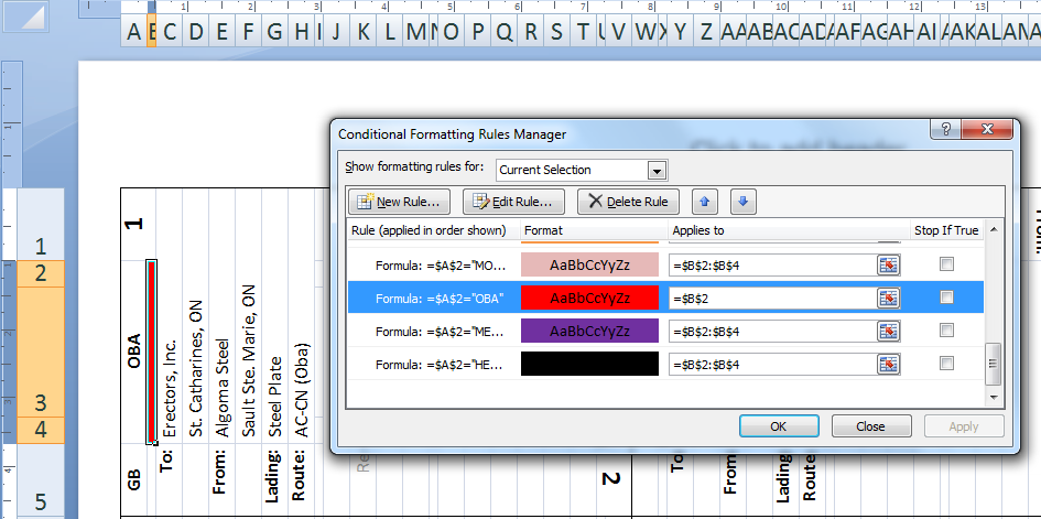
You’ll see that my waybill template includes a block code for switching/routing at the very top, as generally this is the most important information required when switching or handling cars – “Where does this go?” and using a routing or block code at the top of the waybill makes it easier to identify the car’s immediate destination. This is reinforced with a colour-coded bar below the block code which matches the block. (I plan on making a chart of the blocks and a system map readily available to operators in the model railroad’s timetable document.)

To make the colour coded bar, I created a series of Conditional Formatting rules to apply a fill colour to this cell based on the text value in the block code cell above/beside it.
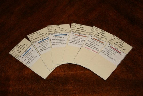
Once the waybill template is completed, it’s a matter of playing around in the data grid to create the various shipment information, and then printing them out in the template by adjusting the starting ID/group to fill in the data and print the results. Cut out with scissors, insert into the appropriate car cards, and voilà:
Files
A few people asked if I would share the actual Excel files. Here they are.
Notes: The car cards file is useable as-is by anyone. I cleared out my own roster information so the entire world doesn’t know my inventory, just leaving the first few cars behind to illustrate how the data works. For the waybills file, I actually uploaded my file as-is, including all my data. Consider it a gift to other ACR modelers, and shows how the data works. Note that if you’re adapting the file to your own railway and want to include the colour coded bars that match to the destination block codes, you’ll have to go in and edit all the conditional formatting rules for your own station/block names. Note that this workbook also contains the customer order sheet described in my previous post.
If clicking on the link doesn’t open the file properly, right click and choose “Save As…” from the menu that comes up. (Mac users with a one-button mouse, I believe you hold the “Command” key and click for this menu.)
Update: see also followup post where I add company logos to the cards.