
Recently I attended an operating session at my club, where we use car cards created and printed from the “ShipIt!” software package. One of the features of the ShipIt! software is the ability to include a railway logo in the top corner of the car card – which I’ve been dully aware of forever since most of our car cards have a CP Rail logo in the upper corner (since our club models CP). However, the guy that prepares and prints out the car cards has actually started using this feature and adding specific logos to cars for different railroads, and the effect is actually pretty sharp when handling the waybills during operations. Thus I got inspired to see if I could add logos to my car cards which I created in Excel. (See my previous post: Excel Car Cards and Waybills)
With a bit of googling, I found this article on ExcelGuru.ca which was exactly what I was looking for. I suggest giving it a read, as this is exactly the information I followed in order to add the logos to my car cards; although I did tweak a couple things in the middle to combine it with my data lookup functions I described in my earlier post on the subject, the original author of that article (Ken Puls) deserves a lot of credit here.
Step 1: Setting up the Image Data
The first section follows the information from the ExcelGuru article pretty much verbatim. We need a new sheet added to the workbook to contain all of the images. Each row in the image table contains two columns, one with the image name, and the second column containing the image pasted into the cell.
![]()
There are basically two ways to go about this: define an image for every railway reporting mark you use in your car cards, or just define each image by itself and add in a separate column to the data sheet to specify the image name for each car card. While the second approach causes you to duplicate some value entries in the data table that drives the car cards, it’s the route I ended up going with so that I could optionally use multiple different images against the same reporting marks in order to display lessee logos on privately owned/leased tank cars and not have to define cells for obscure one-off shortlines and companies that I can’t find logos for.
Note that whatever route you go, every possible value that the data could use *must* be defined in the image table, or you’ll end up with the image cell on the final car card displaying a broken reference. If you define an image for each reporting mark, then each mark must be in the image data sheet, even if there’s no actual for that particular mark. There will just be a blank cell defined for that image. For defining images with names, there should be one “Blank” reference.
Each image doesn’t have to be exactly the same size, but they should all fit into the cell on the car card with at least a pixel or two of white space around the edge or it may actually cut off the card border when printed.
Once the table of images to use has been created, we turn each cell containing an image into a named reference that we can use later.
Highlight the table of cells you created, and then under the “Formulas” tab on the toolbar ribbon, in the “Defined Names” group click on “Create from Selection”. Choose to create names from values in the left column. This will use the names in column A to define a specific name for the corresponding cell in column B that can be used later.
That does it for setting up the image table, now let’s make some use of it.
Step 2: Setting up the Data Cells to drive the Image
The middle bit is where my usage may seem slightly more complicated, as in the example in the article, they link the photo to static text whereas I have yet another layer under this, using VLOOKUP functions (which I got into in detail in my previous post) to retrieve text data from another sheet. However, this really doesn’t affect the instructions much, as really the only difference instead of static text in the “driver” cell, the text is returned by that function.
However I do deviate from the article here a little, so I’ll highlight my steps here. First of course, the new data column is added to the Data sheet to specify the name of the logo image to display on the car card. I skipped creating any data validation on these cells.
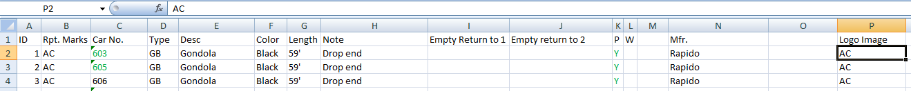
Then, I added a new cell on the car card template page, just below (and outside the printed border of) the finished car card to output the image name using the standard VLOOKUP functions. I also want the cards to print properly if no logo image is specified in the data, so it’s wrapped with an IF function that returns “Blank” if no value is returned, so the picture cell displays a proper blank cell instead of “#REF” indicating a bad lookup. The final cell formula for the first car card on the sheet then looks like this, where cell E16 contains the starting car card ID:
=IF(VLOOKUP(E16,Data!A:P,16,FALSE)="", "Blank", VLOOKUP(E16,Data!A:P,16,FALSE))
Now, select that cell, and use the “Define Name” tool in the “Formulas” tab of the toolbar ribbon to manually set a defined name (e.g. “Car1Picture”) for that cell that will again be referenced later.
Next, click on the Name Manager tool in the same section of the toolbar ribbon. We want to edit the name we created and modify its reference a little. Select the new entry (e.g. “Car1Picture”) and change the “Refers To” from:
='Car Cards'!$A$13
to:
=INDIRECT('Car Cards'!$A$13)
What this does is allow this name to refer not specifically to this cell, but to use the value of this cell to refer to another cell, which will allow us to look up the correct cell in the Images table based on the changing sheet data.
Step 3: Linking and Displaying the Image
The final steps are again pretty much followed exactly as presented in the posting on ExcelGuru.
On the Images sheet, select the *cell* (not the actual image object) for the first image and press Ctrl-C to copy it.
Then on the car card template sheet, select the cell where the logo will go and paste in a picture link. It’s important to pick the correct paste option here. The ExcelGuru article shows how to do it in Excel 2010 (right click in the cell, and from the pop-up menu choose Paste Special > Picture Link (icon at bottom right like a little landscape picture with a chain link in front of it)). In the older Excel 2007, which I have, select the cell, and then under the “Home” tab of the toolbar click on Paste > As Picture > Paste Picture Link. This creates a picture object that displays a view of the linked cell.
Of course the point is for it to change based on the sheet data, and not just display the same picture, so we want to change the reference. Click on the created picture to select it, and in the formula bar change the reference to the named cell (from Step 2) that contains the image name for this car card:
![]()
And presto! The car card now has an image that will change based on the data for the car card. The final result looks something like this:

Files
If you’d like to print your own car cards, here’s an almost-blank copy of my Excel template, with just a few sample cars as data examples.
This is outstanding, thank you!